Post-processing with QGIS

During a hydraulic study, we want to visualize simulations results directly over the study area. This tutorial presents a method for visualizing Watlab simulation results using QGIS. ## Importing Watlab result files into QGIS For each simulated time step, Watlab generates a pic_XX_XX.txt file containing the results, typically stored in a folder named Output. These files can be imported into QGIS as point layers.

Open QGIS and go to: Layer → Add Layer → Add Delimited Text Layer...

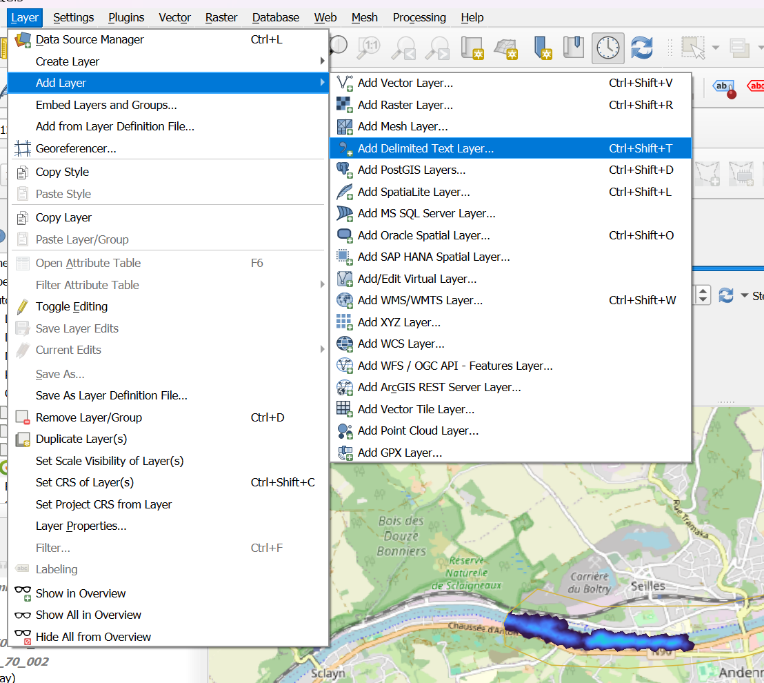
Parameters: - File name: Click the three dots to browse to your Output folder and select the pic_XX_XX.txt file corresponding to the desired time step. - File format: Choose “Custom delimiter” and select Tab. - Sample Data: Make sure the columns are correctly detected (e.g., x, y, zb, h, etc.). - Geometry definition:

- Type: Point

- X field: x

- Y field: y

- Coordinate reference system: Lambert 72 (EPSG:31370)

Once the layer is added, you should see a cloud of points representing the model mesh, one point per cell.

Interpolating results into a raster (TIF File)

To visualize the results as a continuous surface, interpolate the point data into a raster.

Open the Processing Toolbox:

Processing Toolbox → TIN Interpolation

Parameters: - Vector layer: Select the pic layer imported earlier. - Interpolation attribute: Choose h_zb, click the + to add it. - Interpolation method: Linear - Extent: Use the extent of the pic layer. - Pixel size: Set according to the desired resolution.

Give the TIF file a clear name to identify the time step and variable. In the layer properties, adjust the symbology for optimal readability.

💡 To produce high-quality visual outputs, QGIS also allows you to design map layouts with legends, titles, and scale bars using ``Project`` → ``New Print Layout``. This is ideal for exporting clean figures for reports or presentations.

Elevation profile

To represent water surface elevation relative to terrain, you need to combine the water depth h with the terrain elevation zb from the model. This allows you to create elevation profiles.

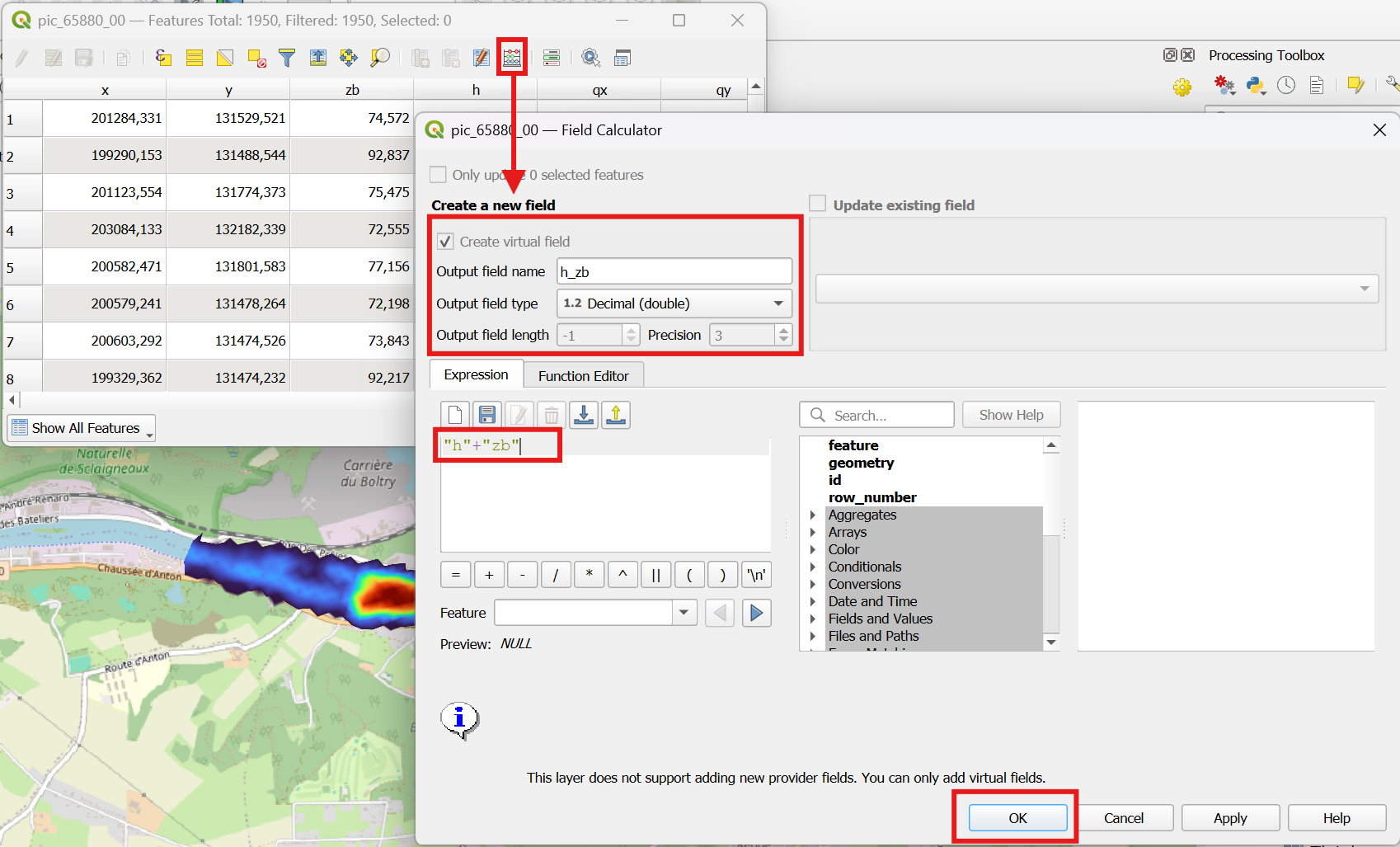
First, add a new column h_zb to the attribute table of your result file.

1. Open the attribute table of the pic_XX_XX.txt layer (right-click on the layer → Open Attribute Table).

2. Open the Field Calculator:

   • Create a new field

   • Name: h_zb

   • Output file type: Decimal (double)

   • Expression:

     "h" + "zb"
     

3. Apply the calculation.

Next, re-interpolate the results using TIN interpolation, this time using the h_zb attribute.

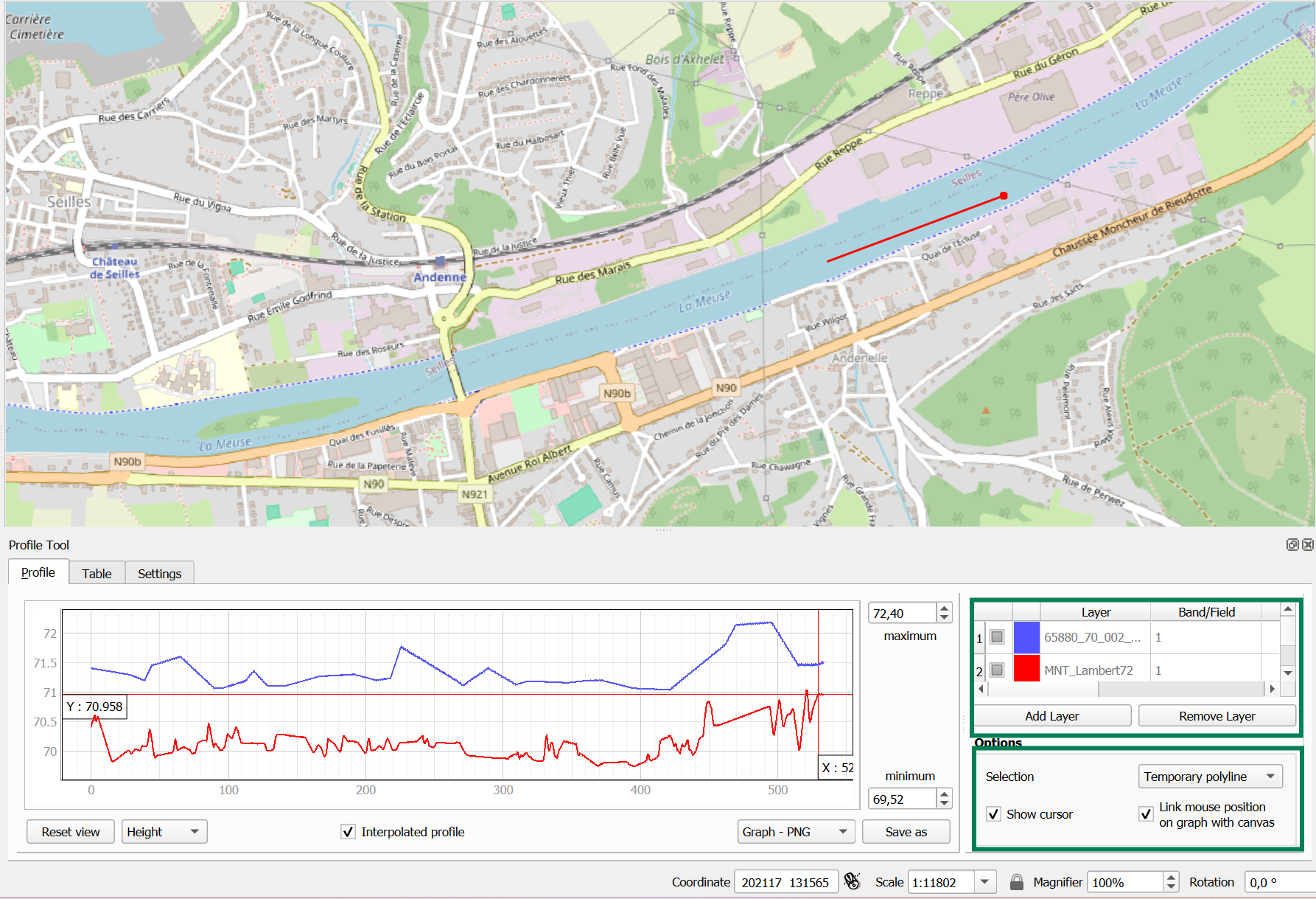
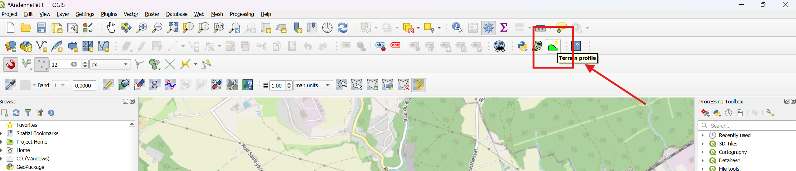
To generate a terrain profile, you can use the Profile Tool plugin. This allows you to draw a temporary line directly on the map or use a predefined shapefile if you want to consistently apply the same cross-section across different datasets.

Once the raster is generated, you can compare the interpolated water level with your DEM to produce elevation profiles at a specific time step.

The picture below illustrates a typical elevation profile:

• Red curve: Digital Elevation Model (DEM), representing the terrain.

• Blue curve: Water surface elevation (h + zb), showing the simulated water level.

💡 You can export the data (right-click → Export) and make beautiful plots using Python libraries.