A comprehensive example

This jupyter notebook is a complete example of how to use Watlab. It will guide you through the different steps of a classic Watlab usage: the mesh creation with GMSH, the model description with one of the modules of Watlab, and the visualisation with the visualisation tools of Watlab.

Now make sure you have installed Watlab correctly, and dig in with us!

All you need is GMSH!

GMSH is a mesh generator. It comes with a GUI, but also with a nice Python-API. The very first step is to import GMSH and initialise the process. Then, we’ll be able to construct the mesh point by point.

# Import the module
import gmsh
import sys

# Initialise gmsh and create a model
gmsh.initialize()
gmsh.model.add("damBreak")

Set up the geometry of the domain

The domain of this first example will look like the picture displayed here under: a rectangle with two separated zones. The left one will be filled with water and called “Filled area”, and the right one will be empty and called “Empty area”.

The domain is made of several physical objects that must be created sequentially. They are part of the geometry of the model.

1. Six points correspond to the nodes of the domain (one at each corner, two in the middle to create the separation line).

The points are just coordinates. To each point, one must specify a mesh-size characteristic. Optionnally, one can give it a number (otherwise, it is set automatically). We recommend to attribute the number manually to control it easily.

#characteristic size of cells
lc = 0.01

# create points
gmsh.model.geo.addPoint(0, 0, 0, lc, 1)
gmsh.model.geo.addPoint(0.5, 0, 0, lc, 2)
gmsh.model.geo.addPoint(1, 0, 0, lc, 3)
gmsh.model.geo.addPoint(0, 0.4, 0, lc, 4)
gmsh.model.geo.addPoint(0.5, 0.4, 0, lc, 5)
gmsh.model.geo.addPoint(1,0.4, 0, lc, 6)

6

2. Seven edges join thoses points: six for the contour, one for the separation

The edges join two points to each other. They also receive each an identifier number. The syntax is extremely simple: addLine(point_i, point_j, line_identifier).

gmsh.model.geo.addLine(1, 2, 1)
gmsh.model.geo.addLine(2, 3, 2)
gmsh.model.geo.addLine(1, 4, 3)
gmsh.model.geo.addLine(2, 5, 4)
gmsh.model.geo.addLine(3, 6, 5)
gmsh.model.geo.addLine(4, 5, 6)
gmsh.model.geo.addLine(5, 6, 7)

7

3. Two curve loops delimit the zones

The curves are concatenation of lines. The orientation is very important here, as the line is defined as coming from point_i and going to point_j. Each curve receives an identifier.

The syntax, again, is simple: addCurveLoop(list_of_lines_identifiers, indentifier).

Warning: every curve loop must be created in counter-clockwise direction. Otherwise, the cells will not be properly oriented.

gmsh.model.geo.addCurveLoop([1, 4, -6, -3], 1)
gmsh.model.geo.addCurveLoop([2, 5, -7, -4], 2)

2

4. Two plane surface represent the zones

Finally, the plane surfaces are build on (one or more) curves, with the syntax addPlaneSurface(list_of_curveLoops_identifiers, identifier).

gmsh.model.geo.addPlaneSurface([1], 1)
gmsh.model.geo.addPlaneSurface([2], 2)

2

Set up the model

Now, that the geometry is set up, one can build the model on it, and give names to objects that we will manipulate later with Watlab. Those objects are named “Physical Groups” and represent the boundaries, or the areas. The basic syntax is: addPhysicalGroup(dimension, list_of_suited_identifiers, name="a nice name")

The groups may be of two types:

1. Boundaries are Physical Groups of dimension one, and build on line identifiers. They are created as addPhysicalGroup(1, list_of_lines_identifiers, name="a nice boundary name")

2. Areas are Physical Groups of dimension two, and build on plane surfaces identifiers. They are created as addPhysicalGroup(2, list_of_plane_surfaces_identifiers, name="a nice zone name").

# first synchronize the information with gmsh.model !
gmsh.model.geo.synchronize()

# Dimension 1 groups (boundaries) build on lines identifiers.
gmsh.model.addPhysicalGroup(1, [1,2],name="Boundaries down")
gmsh.model.addPhysicalGroup(1, [5],name="Boundaries right")
gmsh.model.addPhysicalGroup(1, [6,7],name="Boundaries up")
gmsh.model.addPhysicalGroup(1, [3],name="Boundaries left")

gmsh.model.addPhysicalGroup(1, [4],name="Center line")

# Dimension 2 groups (areas) build on plane surfaces identifiers.
gmsh.model.addPhysicalGroup(2, [1],name="Filled area")
gmsh.model.addPhysicalGroup(2, [2],name="Empty area")

7

Let the magic play!

Now you can generate the mesh and save it with the following commands.

# We generate and optimize the mesh
gmsh.model.mesh.generate(2)
gmsh.model.mesh.optimize('Laplace2D')

# Here we save the mesh as a .msh file
gmsh.write("damBreakMesh.msh")
if '-nopopup' not in sys.argv:
    gmsh.fltk.run()

# And we finalize gmsh.
gmsh.finalize()

Watlab helps you master the model

Now that the geometry of your domain is done, you can focus on solving your hydraulic problem. For this, you need a solver (hopefully, Watlab provides you one!). You also need to tell Watlab what mesh represents the domain, and what conditions are set to the cells and the boundaries.

First, import Watlab, import the mesh, and create a Watlab model!

The example here is hydrodynamics, so the solver is hydroflow.

import watlab

# The mesh is created from the .msh file saved above
mesh = watlab.Mesh("damBreakMesh.msh")

# Impose a meshchecking if needed (defaul = False)
mesh.meshchecking = True

# The model builds on that mesh
model = watlab.HydroflowModel(mesh)

The model can be give several properties (see the documentation for a complete set of properties).

# Your model requires some general parameters such as the simulation time.
model.name = "Simple Dam Break"
model.ending_time = 5
model.Cfl_number = 0.95

But the most interresting functions concern the initial conditions and boundary conditions (check also the doc for a comprehensive list). The conditions are associated with an area from the mesh or a boundary. Just call them by their nice name, and Watlab will find them :-). The syntax is usually: set_certain_condition(list_of_areas_names, list_of_values).

# We specify the friction coefficient to both zones to 0.01
model.set_friction_coefficient("Filled area",0.01)
model.set_friction_coefficient("Empty area",0.01)

# But the initial water height must be different in the filled area than in the empty one.
model.set_initial_water_height("Filled area", 0.15)
model.set_initial_water_height("Empty area", 0.015)

Here, all boundaries are walls, except the center line between the filled and empty areas.

model.set_wall_boundaries(["Boundaries down","Boundaries up","Boundaries left","Boundaries right"])

Finally, we can specify output parameters and generate the data files.

# Here we choose how many "pictures" of the flow we want
model.set_picture_times(n_pic = 51)

# And here we set the names of the io folders (by default, they are named... input and output. How imaginative!)
model.export.input_folder_name = "InputExample01"
model.export.output_folder_name = "OutputExample01"

# Finally, we generate the datafiles needed by the solver.
model.export_data()

The data files are stored in the input folder. They are super important for the solver: without them, no simulation will be run. Speaking of running a simulation, you just need to run the model (the solver can sometimes be parallelized).

model.solve(isParallel=True)

meshchecker.exe exists
Launching the meshchecker executable ...
hydroflow.exe exists
Launching the executable ...
Boundary condition of type 4234 not defined!

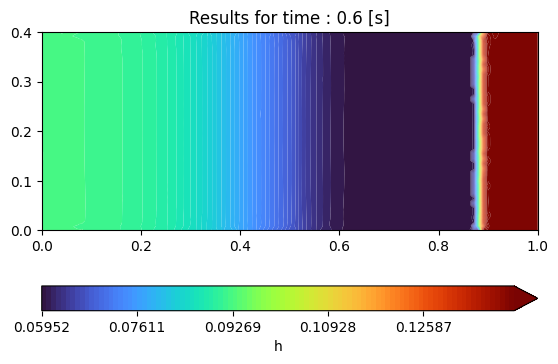
Visualise the outputs thanks to Watlab

Nothing seems to happen? It’s normal. Output files have been outputed in the dedicated folder. Watlab comes with basic visualisation functions to saves you from writing your own plotters.

You need to first create a plotter, then just reference the files of the picture you want to print.

# create a plotter based on the watlab's mesh
import matplotlib.pyplot as plt

plotter = watlab.Plotter(mesh)

# And plot
myPic = "OutputExample01\\pic_0_60.txt"
plotter.plot(myPic,'h')
plt.title("Results for time : 0.6 [s]")
plt.show()