Circular Dam Break

This jupyter notebook is a complete example of how to use Watlab. It will guide you through the different steps of a classic Watlab usage: the mesh creation with GMSH, the model description with one of the modules of Watlab, and the visualisation with the visualisation tools of Watlab.

Now make sure you have installed Watlab correctly, and dig in with us!

In this example, we perform a circular dam break.

All you need is GMSH!

First, lets create the mesh with a circular region at the middle:

import gmsh
import sys

gmsh.initialize()
gmsh.model.add("circularDamBreak")

lc = 0.05
gmsh.model.geo.addPoint(0, 0, 0, lc, 1)
gmsh.model.geo.addPoint(5, 0, 0, lc, 2)
gmsh.model.geo.addPoint(5, 5, 0, lc, 3)
gmsh.model.geo.addPoint(0, 5, 0, lc, 4)
gmsh.model.geo.addPoint(3.25, 2.5, 0, lc, 5)
gmsh.model.geo.addPoint(2.5, 3.25, 0, lc, 6)
gmsh.model.geo.addPoint(1.75, 2.5, 0, lc, 7)
gmsh.model.geo.addPoint(2.5, 1.75, 0, lc, 8)
gmsh.model.geo.addPoint(2.5, 2.5, 0, lc, 9) #center tag

gmsh.model.geo.addLine(1, 2, 1)
gmsh.model.geo.addLine(2, 3, 2)
gmsh.model.geo.addLine(3, 4, 3)
gmsh.model.geo.addLine(4, 1, 4)
gmsh.model.geo.addCircleArc(5,9,6,5)
gmsh.model.geo.addCircleArc(6,9,7,6)
gmsh.model.geo.addCircleArc(7,9,8,7)
gmsh.model.geo.addCircleArc(8,9,5,8)

gmsh.model.geo.addCurveLoop([1, 2, 3, 4], 1)
gmsh.model.geo.addCurveLoop([5, 6, 7, 8], 2)

gmsh.model.geo.addPlaneSurface([1,2], 1)
gmsh.model.geo.addPlaneSurface([2], 2)

gmsh.model.geo.synchronize()

gmsh.model.addPhysicalGroup(1, [1],name="Boundaries down")
gmsh.model.addPhysicalGroup(1, [2],name="Boundaries right")
gmsh.model.addPhysicalGroup(1, [3],name="Boundaries up")
gmsh.model.addPhysicalGroup(1, [4],name="Boundaries left")

gmsh.model.addPhysicalGroup(2, [1],name="Empty Area")
gmsh.model.addPhysicalGroup(2, [2],name="Circular dam")

gmsh.model.mesh.generate(2)
gmsh.model.mesh.optimize('Laplace2D')
gmsh.write("circularDamBreakMesh.msh")
if '-nopopup' not in sys.argv:
    gmsh.fltk.run()

gmsh.finalize()

Watlab helps you master the model

Now that the geometry of your domain is done, you can focus on solving your hydraulic problem. For this, you need a solver (hopefully, Watlab provides you one!). You also need to tell Watlab what mesh represents the domain, and what conditions are set to the cells and the boundaries.

The example here is only hydrodynamics, so the solver is hydroflow.

In this example, we use a the HydroFlow’s API to model another geometrical case. It consists of a circular dambreak happening in a square box.

First, import Watlab, import the mesh, and create a Watlab model!

import watlab
import numpy as np

mesh = watlab.Mesh("circularDamBreakMesh.msh")
model = watlab.HydroflowModel(mesh)

Several properties can be given to the model (see the documentation for a complete set of properties).

model.name = "Circular Dam break"
model.ending_time = 50
model.Cfl_number = 0.95

Initial conditions and physical properties, such as friction coefficient or water level can be given as follows:

model.set_friction_coefficient("Circular dam",0.01)
model.set_friction_coefficient("Empty Area",0.01)
model.set_initial_water_height("Circular dam", 1)

model.set_wall_boundaries(["Boundaries down","Boundaries up","Boundaries left","Boundaries right"])

Provide the number of required results files:

model.set_picture_times(pic_array = np.arange(0,50,1).tolist())

Finally, we can specify output parameters, generate the data files and run this specific model:

model.export_data()
print("Input files generated!")
model.solve()

Input files generated!
hydroflow.exe exists
Launching the executable ...
Total execution time: 177 sec. for 50 sec. of simulation.

Visualize the results with the Plotter class combined with matplotlib

import matplotlib.pyplot as plt

#create the mesh and plotter object
plotter = watlab.Plotter(mesh)

#time of the plot
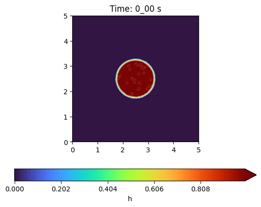
time0 = "0_00"
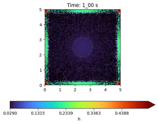
time1 = "1_00"
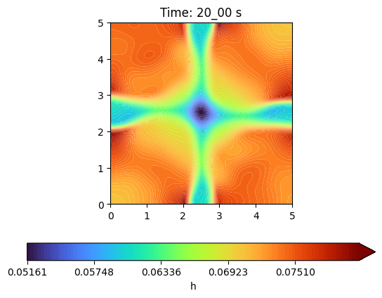
time2 = "20_00"
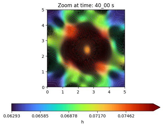
time3 = "40_00"

#path of the pic at the corresponding times
myPic0 = "output\\pic_"+ time0 +".txt"
myPic1 = "output\\pic_"+ time1 +".txt"
myPic2 = "output\\pic_"+ time2 +".txt"
myPic3 = "output\\pic_"+ time3 +".txt"

#plot
plotter.plot(myPic0, "h") #show = false
plt.title("Time: " + time0 +" s")
plt.show()

plotter.plot(myPic1, "h")
plotter.show_velocities(myPic1, scale=100, velocity_ds=0.4)
plt.title("Time: " + time1 +" s")
plt.show()

plotter.plot(myPic2, "h")
plt.title("Time: " + time2 +" s")
plt.show()

plotter.plot(myPic3, "h")
plotter.show_velocities(myPic3, scale=7)
plt.title("Zoom at time: " + time3+" s")
plt.show()

#cross section plot
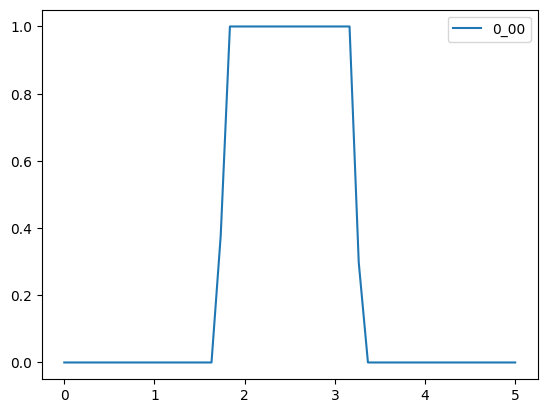
plotter.plot_profile_along_line(myPic0, "h", x_coordinate=[0,5], y_coordinate=[2.5,2.5], new_fig=True, label=time0)