Demo for CoBP
The following matlab code provides a demonstration framework for the methods developed in:
A. Moshtaghpour, L. Jacques, V. Cambareri, K. Degraux, C. De Vleesschouwer, "Consistent Basis Pursuit for Signal and Matrix Estimates in Quantized Compressed Sensing"
This script contains two demonstrations: one for K-sparse signal estimation from quantized observations, the other for rank-1 matrix estimation in QCS.
Authors: A. Moshtaghpour, L. Jacques
July, 2015
Contents
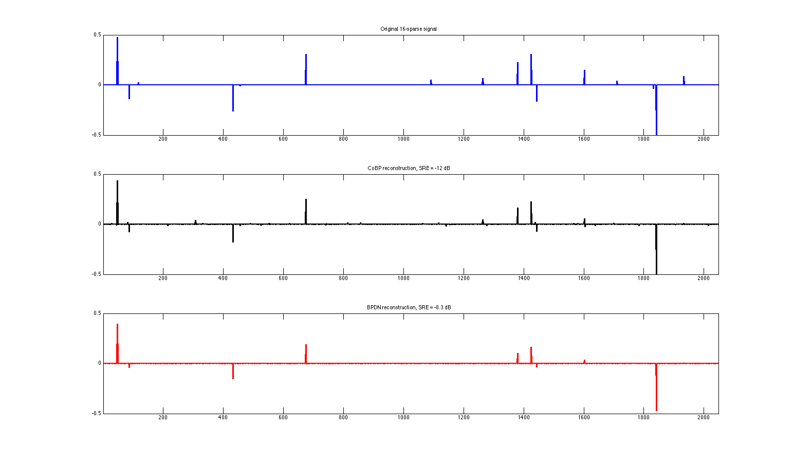
Demo 1: K-sparse signal estimation in QCS
As a first demonstration, we propose to reconstruct sparse signals from their quantized compressive observations.
As mentioned in that paper, two methods are tested here for sparse signals:


where  is the quantized compressive measurements of an initial K-sparse signal
  ,
,  is a
is a  Gaussian Random matrix.
Initializing
addpath('mod_unlocbox');

% Loading toolbox
init_unlocbox()

% Setting solver parameters
param_solver.verbose = 0;          % display parameter
param_solver.maxit = 60000;        % maximum number of iterations
param_solver.tol = 1e-6;           % tolerance to stop iterating
param_solver.gamma = 5e-3;         % proximal operator parameter
Conventions
% Size of the signal
N = 2048;

% Sparsity level
K = 16;

% Number of measurements
M = 64 * K;

% Number of bits
B = 2;

% Quantizer bin width
delta = 6/2^(B-1);

% BPDN l2 error bound
%(see Sec.V: L. Jacques, D. K. Hammond, M. J. Fadili, "Dequantizing compressed sensing")
epsilon = delta * sqrt(M+6*sqrt(M))/(2*sqrt(3));

% Uniform midrise quantizer
Q = @(x,delta) delta*floor(x/delta) + delta/2;
Generating signals and matrices
%  Generating sparse signal with normalized l2 norm
idx = randperm(N);
x = zeros(N,1);
x(idx(1:K)) = randn(K,1);
x = x/norm(x);

%  Generating Gaussian mesurement matrix
Phi = randn(M, N);

%  Generating dithering vector ~U(-delta/2 , delta/2)
dithering = -delta/2+delta*rand(M,1);
Acquiring measurements
%  Compressive measurements
y = Phi * x + dithering;

%  Quantizing the compressive measurements
yq = Q(y,delta);
Solving CoBP and BPDN problems
% BPDN
param_solver.init_pt = zeros(N,1);
xhat_bpdn = func_BPDN(yq-dithering,Phi,epsilon,param_solver);

% CoBP (with a warm start from BPDN solution, works also without)
param_solver.init_pt = xhat_bpdn;
xhat_cobp = func_CoBP(yq-dithering,Phi,delta,param_solver);
SRE calculation
% CoBP
SRE_cobp = 20*log10(norm(x-xhat_cobp));

% BPDN
SRE_bpdn = 20*log10(norm(x-xhat_bpdn));
Plotting the results
figure

% Ground truth signal
subplot(3,1,1)
plot(1:N,x,'b-','linewidth',2)
title(sprintf('Original %i-sparse signal',K))
xlim([1 N])
ylim([-0.5 0.5])

% CoBP reconstructed signal
subplot(3,1,2)
plot(1:N,xhat_cobp,'k-','linewidth',2)
title(sprintf('CoBP reconstruction, SRE = %2.2g dB',SRE_cobp))
xlim([1 N])
ylim([-0.5 0.5])

% BPDN reconstructed signal
subplot(3,1,3)
plot(1:N,xhat_bpdn,'r-','linewidth',2)
title(sprintf('BPDN reconstruction, SRE = %2.2g dB',SRE_bpdn))
xlim([1 N])
ylim([-0.5 0.5])
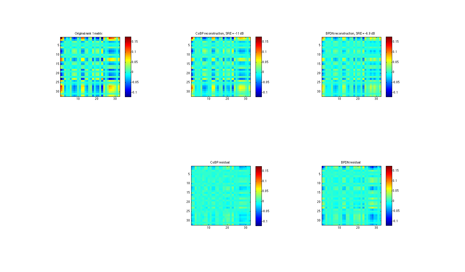
Demo 2: rank-1 matric estimation in QCS
As mentioned in that paper, two methods are tested here for low-rank matrix reconstruction:


where 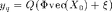 is the quantized compressive measurements of an initial rank-1 matrix
  whose vector representation is
  , is a Gaussian Random matrix.
% Setting solver parameters
param_solver.verbose = 0;          % display parameter
param_solver.maxit = 60000;        % maximum number of iterations
param_solver.tol = 1e-6;           % tolerance to stop iterating
param_solver.gamma = 5e-3;         % proximal operator parameter
Conventions
% Size of the signal
N = 1024;
n = sqrt(N);

% rank of the sensed matrix
r = 1;
P = 64;
% Number of measurements
M = 16 * P;

% Number of bits
B = 2;

% Quantizer bin width
delta = 6/2^(B-1);

% BPDN l2 error bound
%(see Sec.V: L. Jacques, D. K. Hammond, M. J. Fadili, "Dequantizing compressed sensing")
epsilon = delta * sqrt(M+6*sqrt(M))/(2*sqrt(3));

% Uniform midrise quantizer
Q = @(x,delta) delta*floor(x/delta) + delta/2;
Generating signals and matrices
%  Generating rank one matrix with normalized Frobenius norm
x0 = randn(n,1);
X = x0*x0';
X = X/norm(X,'fro');
x = X(:);

%  Generating Gaussian mesurement matrix
Phi = randn(M, N);

%  Generating dithering vector ~U(-delta/2 , delta/2)
dithering = -delta/2+delta*rand(M,1);
Acquiring measurements
%  Compressive measurements
y = Phi * x + dithering;

%  Quantizing the compressive measurements
yq = Q(y,delta);
Solving CoBP and BPDN problems
% BPDN
param_solver.init_pt = zeros(N,1);
xhat_bpdn = func_BPDN_matrix_completion(yq-dithering,Phi,epsilon,param_solver);

% CoBP (with a warm start from BPDN solution, works also without)
param_solver.init_pt = xhat_bpdn;
xhat_cobp = func_CoBP_matrix_completion(yq-dithering,Phi,delta,param_solver);
SRE calculation
% CoBP
SRE_cobp = 20*log10(norm(x-xhat_cobp));

% BPDN
SRE_bpdn = 20*log10(norm(x-xhat_bpdn));
Plotting the results
figure

% Ground truth signal
subplot(2,3,1)
imagesc(reshape(x,[n,n]));
caxis([min(x(:)) max(x(:))])
colorbar;
axis square;
title(sprintf('Original rank %i matrix',r))

% CoBP reconstructed signal
subplot(2,3,2)
imagesc(reshape(xhat_cobp,[n,n]));
caxis([min(x(:)) max(x(:))])
colorbar;
axis square;
title(sprintf('CoBP reconstruction, SRE = %2.2g dB',SRE_cobp))

% BPDN reconstructed signal
subplot(2,3,3)
imagesc(reshape(xhat_bpdn,[n,n]));
caxis([min(x(:)) max(x(:))])
colorbar;
axis square;
title(sprintf('BPDN reconstruction, SRE = %2.2g dB',SRE_bpdn))

% CoBP reconstructed signal
subplot(2,3,5)
imagesc(reshape(xhat_cobp - x,[n,n]));
caxis([min(x(:)) max(x(:))])
colorbar;
axis square;
title('CoBP residual')

% BPDN reconstructed signal
subplot(2,3,6)
imagesc(reshape(xhat_bpdn - x,[n,n]));
caxis([min(x(:)) max(x(:))])
colorbar;
axis square;
title('BPDN residual')

% Closing the toolbox
close_unlocbox();